D Reproducible analysis and workflow
The notion that scientific findings can be confirmed repeatedly through replication is fundamental to the centuries-old paradigm of science. The underlying logic is that if you have identified a truth about the world, that truth should persist upon further investigation by other observers. In the physical sciences, there are two challenges in replicating a study: replicating the experiment itself, and reproducing the subsequent data analysis that led to the conclusion. More concisely, replicability means that different people get the same results with different data. Reproducibility means that the same person (or different people) get the same results with the same data.
It is easy to imagine why replicating a physical experiment might be difficult, and not being physical scientists ourselves, we won’t tackle those issues here. On the other hand, the latter challenge of reproducing the data analysis is most certainly our domain. It seems like a much lower hurdle to clear—isn’t this just a matter of following a few steps? Upon review, for a variety of reasons many scientists are in fact tripping over even this low hurdle.
To further explicate the distinction between replicability and reproducibility, recall that scientists are legendary keepers of lab notebooks. These notebooks are intended to contain all of the information needed to carry out the study again (i.e., replicate): reagents and other supplies, equipment, experimental material, etc. Modern software tools enable scientists to carry this same ethos to data analysis: Everything needed to repeat the analysis (i.e., reproduce) should be recorded in one place.
Even better, modern software tools allow the analysis to be repeated at the push of a button. This provides a proof that the analysis being documented is in fact exactly the same as the analysis that was performed. Moreover, this capability is a boon to those generating the analysis. It enables them to draft and redraft the analysis until they get it exactly right. Even better, when the analysis is written appropriately, it’s straightforward to apply the analysis to new data. Spreadsheet software, despite its popularity, is not suitable for this. Spreadsheet software references specific rows and columns of data, and so the analysis commands themselves need to be updated to conform to new data.
The replication crisis is a very real problem for modern science. More than 15 years ago, Ioannidis (2005) argued that “most published research findings are false.” More recently, the journal Nature ran a series of editorials bemoaning the lack of replicability in published research (Editorial 2013). It now appears that even among peer-reviewed, published scientific articles, many of the findings—which are supported by experimental and statistical evidence—do not hold up under the scrutiny of replication. That is, when other researchers try to do the same study, they don’t reliably reach the same conclusions.
Some of the issues leading to irreproducibility are hard to understand, let alone solve. Much of the blame involves multiplicity and the “garden of forking paths” introduced in Chapter 9. While we touch upon issues related to null hypothesis testing in Chapter 9, the focus of this chapter is on modern workflows for reproducible analysis, since the ability to regenerate a set of results at a later point in time is a necessary but not sufficient condition for reproducible results.
The National Academies report on undergraduate data science included workflow and reproducibility as an important part of data acumen (National Academies of Science, Engineering, and Medicine 2018). They described key components including workflows and workflow systems, reproducible analysis, documentation and code standards, version control systems, and collaboration.
Reproducible workflows consist of three components: a fully scriptable statistical programming environment (such as R or Python), reproducible analysis (first described as literate programming), and version control (commonly implemented using GitHub).
D.1 Scriptable statistical computing
In order for data analysis to be reproducible, all of the steps taken in the analysis have to be recorded in a linear fashion. Scriptable applications like Python, R, SAS, and Stata do this by default. Even when graphical user interfaces to these programs are used, they add the automatically-generated code to the history so that it too can be recorded. Thus, the full series of commands that make up the data analysis can be recorded, reviewed, and transmitted. Contrast this with the behavior of spreadsheet applications like Microsoft Excel and Google Sheets, where it is not always possible to fully retrace one’s steps.
D.2 Reproducible analysis with R Markdown
The concept of literate programming was introduced by Knuth decades ago (Knuth 1992). His advice was:
“Instead of imagining that our main task is to instruct a computer what to do, let us concentrate rather on explaining to human beings what we want a computer to do.”
Central to this prescription is the idea that the relevant documentation for the code—which is understandable not just to the programmer, but to other human beings as well—occurs alongside the code itself. In data analysis, this is manifest as the need to have three kinds of things in one document: the code, the results of that code, and the written analysis. We belong to a growing group of people who find the rmarkdown (J. J. Allaire et al. 2014) and knitr packages (Y. Xie 2014) to be an environment that is ideally suited to support a reproducible analysis workflow (B. S. Baumer et al. 2014).
The rmarkdown and knitr packages use a source file and output file paradigm. This approach is common in programming but is fundamentally different than a “what-you-see-is-what-you-get” editor like Microsoft Word or Google Docs. Code is typed into the source document, which is then rendered into an output format that is readable by anyone. The principles of literate programming stipulate that the source file should also be readable by anyone.
We favor the simple document markup language R Markdown (J. Allaire et al. 2020) for most applications. An R Markdown source file can be rendered (by knitr, leveraging pandoc) into PDF, HTML, and Microsoft Word formats. The resulting document will contain the R code, the results of that code, and the analyst’s written analysis.
Markdown is well-integrated with RStudio, and both LaTeX and Markdown source files can be rendered via a single-click mechanism. More details can be found in Y. Xie (2014) and Gandrud (2014) as well as the CRAN reproducible research task view (Kuhn 2020). See also (http://yihui.name/knitr).
As an example of how these systems work, we demonstrate a document written in the Markdown format
using data from the
SwimRecords data frame. Within RStudio, a new template R Markdown file can be generated by selecting R Markdown from the New File option on the File menu. This generates the dialog box displayed in Figure
D.1. The default output format is HTML, but other options (PDF or Microsoft Word) are available.
The Markdown templates included with some packages (e.g., mosaic) are useful to set up more appropriate defaults for figure and font size. These can be accessed using the “From Template” option when opening a new Markdown file.
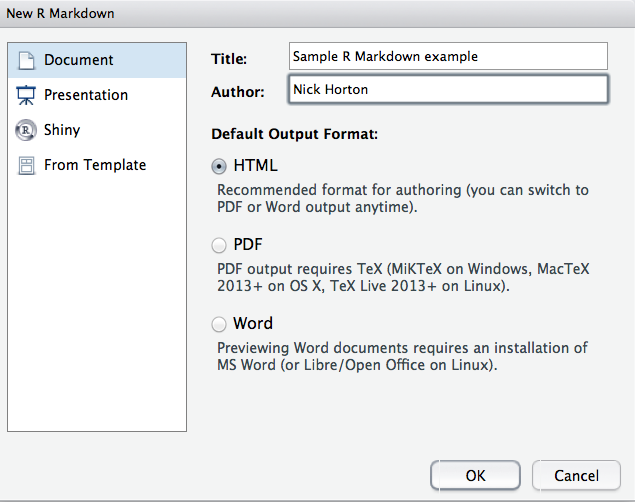
Figure D.1: Generating a new R Markdown file in RStudio.
---
title: "Sample R Markdown example"
author: "Sample User"
date: "November 8, 2020"
output:
  html_document: default
    fig_height: 2.8
    fig_width: 5
---

```{r setup, include=FALSE}
knitr::opts_chunk$set(echo = TRUE)
library(tidyverse)
library(mdsr)
library(mosaic)
```

## R Markdown

This is an R Markdown document. Markdown is a simple formatting syntax for
authoring HTML, PDF, and MS Word documents. For more details on using R
Markdown see http://rmarkdown.rstudio.com.

When you click the **Knit** button a document will be generated that
includes both content as well as the output of any embedded R code chunks
within the document. You can embed an R code chunk like this:

```{r display}
glimpse(SwimRecords)
```

## Including Plots

You can also embed plots, for example:

```{r scatplot, echo=FALSE, message = FALSE}
ggplot(
  data = SwimRecords,
  aes(x = year, y = time, color = sex)
) +
  geom_point() +
  geom_smooth(method = loess, se = FALSE) +
  theme(legend.position = "right") +
  labs(title = "100m Swimming Records over time")
```

There are n=`r nrow(SwimRecords)` rows in the Swim records dataset.

Note that the `echo = FALSE` option was added to the code chunk to
prevent printing of the R code that generated the plot.
Figure D.2: Sample Markdown input file.
Figure D.2 displays a modified version of the default R Markdown input file.
The file is given a title (Sample R Markdown example) with output format set by default to HTML.
Simple markup (such as bolding) is added through use of the ** characters before and after the word Help.
Blocks of code are begun using a ```{r} line and closed
with a ``` line (three back quotes in both cases).
The formatted output can be generated and displayed by clicking the Knit HTML button in RStudio, or by using the commands in the following code block, which can also be used when running R without the benefit of RStudio.
library(rmarkdown)
render("filename.Rmd")   # creates filename.html
browseURL("filename.html")
The render() function extracts the R commands from a specially formatted R Markdown
input file (filename.Rmd), evaluates them, and integrates the resulting output, including text and graphics, into an output file (filename.html).
A screenshot of the results of performing these steps on the .Rmd file displayed in Figure D.2 is displayed in Figure D.3.
render() uses the value of the output: option to determine what format to generate. If the .Rmd file specified output: word_document, then a Microsoft Word document
would be created.
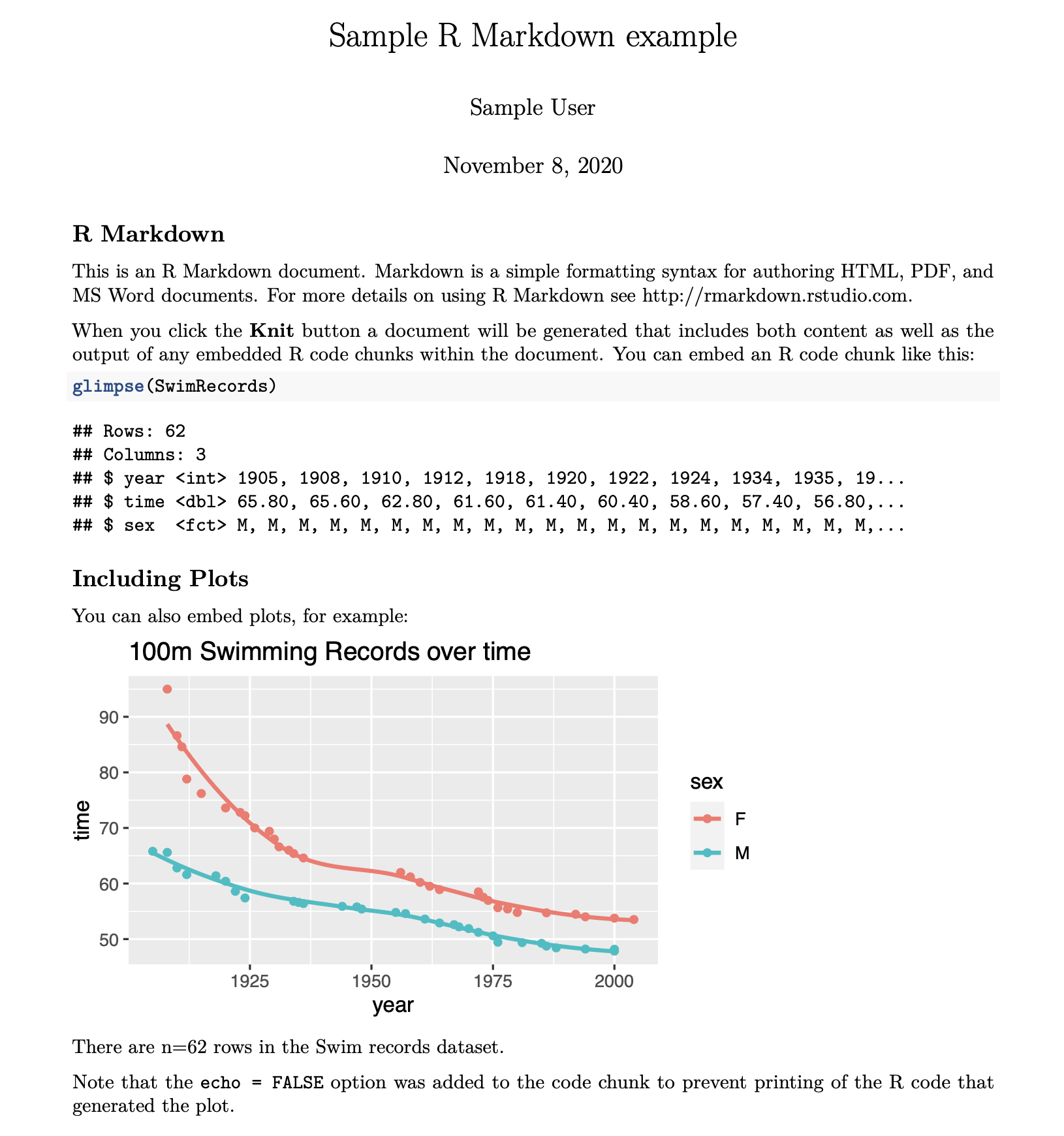
Figure D.3: Formatted output from R Markdown example.
Alternatively, a PDF or Microsoft Word document can be generated in RStudio by selecting New from the R Markdown menu, then clicking on the PDF or Word options.
RStudio also supports the creation of R Presentations using a variant of the R Markdown syntax. Instructions and an example can be found by opening a new R presentations document in RStudio.
D.3 Projects and version control
Projects are a useful feature of RStudio. A project provides a separate workspace. Selecting a project also reorients your RStudio environment to a specified directory, in the process reorienting the Files tab, the working directory, etc. Once you start working on multiple projects, being able to switch back and forth becomes very helpful.
Given that data science has been called a “team sport,” the ability to track changes to files and discuss issues in a collaborative manner is an important prerequisite to reproducible analysis. Projects can be tied to a version control system, such as Subversion or GitHub. These systems help you and your collaborators keep track of changes to files, so that you can go back in time to review changes to previous pieces of code, compare versions, and retrieve older versions as needed.
While critical for collaboration with others, source code version control systems are also useful for individual projects because they document changes and maintain version histories. In such a setting, the collaboration is with your future self!
GitHub is a cloud-based implementation of Git that is tightly integrated into RStudio. It works efficiently, without cluttering your workspace with duplicate copies of old files or compressed archives. RStudio users can collaborate on projects hosted on GitHub without having to use the command line. This has proven to be an effective way of ensuring a consistent, reproducible workflow, even for beginners. This book was written collaboratively through a private repository on GitHub, just as the mdsr package is maintained in a public repository.
Finally, random number seeds (see section 13.6.3) are an important part of a reproducible workflow. It is a good idea to set a seed to allow others (or yourself) to be able to reproduce a particular analysis that has a stochastic component to it.
D.4 Further resources
Project TIER is an organization at Haverford College that has developed a protocol (Ball and Medeiros 2012) for reproducible research. Their efforts originated in the social sciences using Stata but have since expanded to include R.
R Markdown is under active development. For the latest features see the R Markdown authoring guide at (http://rmarkdown.rstudio.com). The RStudio cheat sheet serves as a useful reference.
Broman and Woo (2018) describe best practices for organizing data in spreadsheets.
GitHub can be challenging to learn but is now the default in many data science research settings. Jenny Bryan’s resources on Happy Git and GitHub for the useR are particularly relevant for new data scientists beginning to use GitHub (Bryan, the STAT 545 TAs, and Hester 2018).
Another challenge for reproducible analysis is ever-changing versions of R and other R packages. The packrat and renv packages help ensure that projects can maintain a particular version of R and set of packages. The reproducible package provides a set of tools to enhance reproducibility.
D.5 Exercises
Problem 1 (Easy): Insert a chunk in an R Markdown document that generates an error. Set the options so that the file renders even though there is an error. (Note: Some errors are easier to diagnose if you can execute specific R statements during rendering and leave more evidence behind for forensic examination.)
Problem 2 (Easy): Why does the mosaic package plain R Markdown template include the code chunk option message=FALSE when the mosaic package is loaded?
Problem 3 (Easy): Consider an R Markdown file that includes the following code chunks. What will be output when this file is rendered?
```{r}
x <- 1:5
```
```{r}
x <- x + 1
``````{r}
x
```Problem 4 (Easy): Consider an R Markdown file that includes the following code chunks. What will be output when the file is rendered?
```{r echo = FALSE}
x <- 1:5
```
```{r echo = FALSE}
x <- x + 1
``````{r include = FALSE}
x
```Problem 5 (Easy): Consider an R Markdown file that includes the following code chunks.
What will be output when this file is rendered?
```{r echo = FALSE}
x <- 1:5
```
```{r echo = FALSE}
x <- x + 1
``````{r echo = FALSE}
x
```Problem 6 (Easy): Consider an R Markdown file that includes the following code chunks. What will be output when the file is rendered?
```{r echo = FALSE}
x <- 1:5
```
```{r echo = FALSE, eval = FALSE}
x <- x + 1
``````{r echo = FALSE}
x
```Problem 7 (Easy): Describe in words what the following excerpt from an R Markdown file will display when rendered.
$\hat{y} = \hat{\beta}_0 + \hat{\beta}_1 \cdot x + \epsilon$Problem 8 (Easy): Create an RMarkdown file that uses an inline call to R to display the value of an object that you have created previously in that file.
Problem 9 (Easy): Describe the implications of changing warning=TRUE to warning=FALSE in the following code chunk.
sqrt(-1)Warning in sqrt(-1): NaNs produced[1] NaNProblem 10 (Easy): Describe how the fig.width and fig.height chunk options can be used to control the size of graphical figures.
Generate two versions of a figure with different options.
Problem 11 (Medium): The knitr package allows the analyst to display nicely formatted
tables and results when outputting to pdf files.
Use the following code chunk as an example to create a similar display using your own data.
library(mdsr)
library(mosaicData)
mod <- broom::tidy(lm(cesd ~ mcs + sex, data = HELPrct))
knitr::kable(
  mod,
  digits = c(0, 2, 2, 2, 4),
  caption = "Regression model from HELP clinical trial.",
  longtable = TRUE
)| term | estimate | std.error | statistic | p.value |
|---|---|---|---|---|
| (Intercept) | 55.79 | 1.31 | 42.62 | 0.0000 |
| mcs | -0.65 | 0.03 | -19.48 | 0.0000 |
| sexmale | -2.95 | 1.01 | -2.91 | 0.0038 |
Problem 12 (Medium): Explain what the following code chunks will display and why this might be useful for technical reports from a data science project.
```{r chunk1, eval = TRUE, include = FALSE}
x <- 15
cat("assigning value to x.\n")
```
```{r chunk2, eval = TRUE, include = FALSE}
x <- x + 3
cat("updating value of x.\n")
``````{r chunk3, eval = FALSE, include = TRUE}
cat("x =", x, "\n")
``````{r chunk1, eval = FALSE, include = TRUE}
``````{r chunk2, eval = FALSE, include = TRUE}
```D.6 Supplementary exercises
Available at https://mdsr-book.github.io/mdsr2e/ch-reproducible.html#reproducible-online-exercises
No exercises found