Calculators free human beings from having to perform arithmetic computations by hand. Similarly, programming languages free humans from having to perform iterative computations by re-running chunks of code, or worse, copying-and-pasting a chunk of code many times, while changing just one or two things in each chunk.
For example, in Major League Baseball there are 30 teams, and the game has been played for over 100 years. There are a number of natural questions that we might want to ask about each team (e.g., which player has accrued the most hits for that team?) or about each season (e.g., which seasons had the highest levels of scoring?). If we can write a chunk of code that will answer these questions for a single team or a single season, then we should be able to generalize that chunk of code to work for all teams or seasons. Furthermore, we should be able to do this without having to re-type that chunk of code. In this section, we present a variety of techniques for automating these types of iterative operations.
7.1 Vectorized operations
In every programming language that we can think of, there is a way to write a loop. For example, you can write a for() loop in R the same way you can with most programming languages. Recall that the Teams data frame contains one row for each team in each MLB season.
What might not be immediately obvious is that columns 15 through 40 of this data frame contain numerical data about how each team performed in that season. To see this, you can execute the str() command to see the structure of the data frame, but we suppress that output here. For data frames, a similar alternative that is a little cleaner is glimpse().
str(Teams)glimpse(Teams)
Suppose you are interested in computing the averages of these 26 numeric columns. You don’t want to have to type the names of each of them, or re-type the mean() command 26 times. Seasoned programmers would identify this as a situation in which a loop is a natural and efficient solution. A for() loop will iterate over the selected column indices.
           R           AB            H          X2B          X3B           HR
 681.8147783 5135.6062397 1339.4696223  229.4735632   45.2180624  107.4197044
          BB           SO           SB           CS          HBP           SF
 474.1435140  774.3248597  109.1736301   46.0248419   46.5675676   43.9780585
          RA           ER          ERA           CG          SHO           SV
 681.8137931  575.1353038    3.8466831   46.6318555    9.5461412   24.7527094
      IPouts           HA          HRA          BBA          SOA            E
4019.0472906 1339.2535304  107.4197044  474.4853859  773.7185550  178.8942529
          DP           FP
 134.8357964    0.9667251
This certainly works. However, there are a number of problematic aspects of this code (e.g., the use of multiple magic numbers like 14, 15, and 40). The use of a for() loop may not be ideal. For problems of this type, it is almost always possible (and usually preferable) to iterate without explicitly defining a loop. R programmers prefer to solve this type of problem by applying an operation to each element in a vector. This often requires only one line of code, with no appeal to indices.
It is important to understand that the fundamental architecture of R is based on vectors. That is, in contrast to general-purpose programming languages like C++ or Python that distinguish between single items—like strings and integers—and arrays of those items, in R a “string” is just a character vector of length 1. There is no special kind of atomic object. Thus, if you assign a single “string” to an object, R still stores it as a vector.
a <-"a string"class(a)
[1] "character"
is.vector(a)
[1] TRUE
length(a)
[1] 1
As a consequence of this construction, R is highly optimized for vectorized operations (see Appendix B for more detailed information about R internals). Loops, by their nature, do not take advantage of this optimization. Thus, R provides several tools for performing loop-like operations without actually writing a loop. This concept can be a challenging hurdle for those who are used to more general-purpose programming languages.
Helpful Tip
Try to avoid writing for() loops, even when it seems like the easiest solution.
Many functions in R are vectorized. This means that they will perform an operation on every element of a vector by default. For example, many mathematical functions (e.g., exp()) work this way.
exp(1:3)
[1] 2.718282 7.389056 20.085537
Note that vectorized functions like exp() take a vector as an input, and return a vector of the same length as an output.
This is importantly different behavior than so-called summary functions, which take a vector as an input, and return a single value. Summary functions (e.g., mean()) are commonly useful within a call to summarize(). Note that when we call mean() on a vector, it only returns a single value no matter how many elements there are in the input vector.
mean(1:3)
[1] 2
Other functions in R are not vectorized. They may assume an input that is a vector of length one, and fail or exhibit strange behavior if given a longer vector. For example, if() throws a warning if given a vector of length more than one.
if (c(TRUE, FALSE)) {cat("This is a great book!")}
Error in if (c(TRUE, FALSE)) {: the condition has length > 1
As you get more comfortable with R, you will develop intuition about which functions are vectorized. If a function is vectorized, you should make use of that fact and not iterate over it. The code below shows that computing the exponential of the first 10,000 integers by appealing to exp() as a vectorized function is much, much faster than using map_dbl() to iterate over the same vector. The results are identical.
Try to always make use of vectorized functions before iterating an operation.
7.2 Using across() with dplyr functions
The mutate() and summarize() verbs described in Chapter 4 can take advantage of an adverb called across() that applies operations programmatically. In the example above, we had to observe that columns 15 through 40 of the Teams data frame were numeric, and hard-code those observations as magic numbers. Rather than relying on these observations to identify which variables are numeric—and therefore which variables it makes sense to compute the average of—we can use the across() function to do this work for us. The chunk below will compute the average values of only those variables in Teams that are numeric.
Teams |>summarize(across(where(is.numeric), function(x) mean(x, na.rm =TRUE) ) )
    yearID     Rank        G    Ghome        W        L        R       AB
1 1960.118 4.018062 150.2424 78.11565 74.73695 74.73695 681.8148 5135.606
        H      X2B      X3B       HR       BB       SO       SB       CS
1 1339.47 229.4736 45.21806 107.4197 474.1435 774.3249 109.1736 46.02484
       HBP       SF       RA       ER      ERA       CG      SHO       SV
1 46.56757 43.97806 681.8138 575.1353 3.846683 46.63186 9.546141 24.75271
    IPouts       HA      HRA      BBA      SOA        E       DP        FP
1 4019.047 1339.254 107.4197 474.4854 773.7186 178.8943 134.8358 0.9667251
  attendance      BPF      PPF
1    1395655 100.1862 100.2095
Note that this result included several variables (e.g., yearID, attendance) that were outside of the range we defined previously.
The across() adverb allows us to specify the set of variables that summarize() includes in different ways. In the example above, we used the predicate functionis.numeric() to identify the variables for which we wanted to compute the mean. In the following example, we compute the mean of yearID, a series of variables from R (runs scored) to SF (sacrifice flies) that apply only to offensive players, and the batting park factor (BPF). Since we are specifying these columns without the use of a predicate function, we don’t need to use where() though we need to construct a function on the fly.
Teams |>summarize(across(c(yearID, R:SF, BPF), \(x) mean(x, na.rm =TRUE)))
    yearID        R       AB       H      X2B      X3B       HR       BB
1 1960.118 681.8148 5135.606 1339.47 229.4736 45.21806 107.4197 474.1435
        SO       SB       CS      HBP       SF      BPF
1 774.3249 109.1736 46.02484 46.56757 43.97806 100.1862
The across() function behaves analogously with mutate(). It provides an easy way to perform an operation on a set of variables without having to type or copy-and-paste the name of each variable.
7.3 The map() family of functions
More generally, to apply a function to each item in a list or vector, or the columns of a data frame1, use map() (or one of its type-specific variants). This is the main function from the purrr package. For this example, we calculate the mean of each of the statistics defined above, all at once. Compare this to the for() loop written above. Which is syntactically simpler? Which expresses the ideas behind the code more succinctly?
Teams |>select(15:40) |>map_dbl(mean, na.rm =TRUE)
           R           AB            H          X2B          X3B           HR
 681.8147783 5135.6062397 1339.4696223  229.4735632   45.2180624  107.4197044
          BB           SO           SB           CS          HBP           SF
 474.1435140  774.3248597  109.1736301   46.0248419   46.5675676   43.9780585
          RA           ER          ERA           CG          SHO           SV
 681.8137931  575.1353038    3.8466831   46.6318555    9.5461412   24.7527094
      IPouts           HA          HRA          BBA          SOA            E
4019.0472906 1339.2535304  107.4197044  474.4853859  773.7185550  178.8942529
          DP           FP
 134.8357964    0.9667251
The first argument to map_dbl() is the thing that you want to do something to (in this case, a data frame). The second argument specifies the name of a function (the argument is named .f). Any further arguments are passed as options to .f. Thus, this command applies the mean() function to the 15th through the 40th columns of the Teams data frame, while removing any NAs that might be present in any of those columns. The use of the variant map_dbl() simply forces the output to be a vector of type double.2
Of course, we began by taking the subset of the columns that were all numeric values. If you tried to take the mean() of a non-numeric vector, you would get a warning (and a value of NA).
Teams |>select(teamID) |>map_dbl(mean, na.rm =TRUE)
Warning in mean.default(.x[[i]], ...): argument is not numeric or logical:
returning NA
teamID
    NA
If you can solve your problem using across() and/or where() as described in Section 7.2, that is probably the cleanest solution. However, we will show that the map() family of functions provides a much more general set of capabilities.
7.4 Iterating over a one-dimensional vector
7.4.1 Iterating a known function
Often you will want to apply a function to each element of a vector or list. For example, the baseball franchise now known as the Los Angeles Angels of Anaheim has gone by several names during its history.
# A tibble: 4 × 4
  teamID name                          began ended
  <fct>  <chr>                         <int> <int>
1 LAA    Los Angeles Angels             1961  1964
2 CAL    California Angels              1965  1996
3 ANA    Anaheim Angels                 1997  2004
4 LAA    Los Angeles Angels of Anaheim  2005  2023
Here we specify the option .groups = "drop" because we have now finished with the need to group the resulting tibble.
The franchise began as the Los Angeles Angels (LAA) in 1961, then became the California Angels (CAL) in 1965, the Anaheim Angels (ANA) in 1997, before taking their current name (LAA again) in 2005. This situation is complicated by the fact that the teamIDLAA was re-used. This sort of inconsistent naming is unfortunately common in many data sets.
Now, suppose we want to find the length, in number of characters, of each of those team names. We could check each one manually using the function nchar():
But this would grow tiresome if we had many names. It would be simpler, more efficient, more elegant, and scalable to apply the function nchar() to each element of the vector angel_names. We can accomplish this using map_int(). map_int() is like map() or map_dbl(), but it always returns an integer vector.
map_int(angels_names, nchar)
[1] 18 17 14 29
The key difference between map_int() and map() is that the former will always return an integer vector, whereas the latter will always return a list. Recall that the main difference between lists and data.frames is that the elements (columns) of a data.frame have to have the same length, whereas the elements of a list are arbitrary. So while map() is more versatile, we usually find map_int() or one of the other variants to be more convenient when appropriate.
Helpful Tip
It’s often helpful to use map() to figure out what the return type will be, and then switch to the appropriate type-specific map() variant.
This section was designed to illustrate how map() can be used to iterate a function over a vector of values. However, the choice of the nchar() function was a bit silly, because nchar() is already vectorized. Thus, we can use it directly!
nchar(angels_names)
[1] 18 17 14 29
7.4.2 Iterating an arbitrary function
One of the most powerful uses of iteration is that you can apply any function, including a function that you have defined (see Appendix C for a discussion of how to write user-defined functions). For example, suppose we want to display the top-5 seasons in terms of wins for each of the Angels teams.
We can now do this for each element of our vector with a single call to map(). Note how we named the data argument to ensure that the team_name argument was the one that accepted the value over which we iterated.
angels_names |>map(top5, data = Teams)
[[1]]
  teamID yearID  W  L               name
1    LAA   1962 86 76 Los Angeles Angels
2    LAA   1964 82 80 Los Angeles Angels
3    LAA   1961 70 91 Los Angeles Angels
4    LAA   1963 70 91 Los Angeles Angels

[[2]]
  teamID yearID  W  L              name
1    CAL   1982 93 69 California Angels
2    CAL   1986 92 70 California Angels
3    CAL   1989 91 71 California Angels
4    CAL   1985 90 72 California Angels
5    CAL   1979 88 74 California Angels

[[3]]
  teamID yearID  W  L           name
1    ANA   2002 99 63 Anaheim Angels
2    ANA   2004 92 70 Anaheim Angels
3    ANA   1998 85 77 Anaheim Angels
4    ANA   1997 84 78 Anaheim Angels
5    ANA   2000 82 80 Anaheim Angels

[[4]]
  teamID yearID   W  L                          name
1    LAA   2008 100 62 Los Angeles Angels of Anaheim
2    LAA   2014  98 64 Los Angeles Angels of Anaheim
3    LAA   2009  97 65 Los Angeles Angels of Anaheim
4    LAA   2005  95 67 Los Angeles Angels of Anaheim
5    LAA   2007  94 68 Los Angeles Angels of Anaheim
Alternatively, we can collect the results into a single data frame by using the map_dfr() function, which combines the data frames by row. Below, we do this and then compute the average number of wins in a top-5 season for each Angels team name. Based on these data, the Los Angeles Angels of Anaheim has been the most successful incarnation of the franchise, when judged by average performance in the best five seasons.
`summarise()` has grouped output by 'teamID'. You can override using the
`.groups` argument.
# A tibble: 4 × 4
# Groups:   teamID [3]
  teamID name                              N mean_wins
  <fct>  <chr>                         <int>     <dbl>
1 LAA    Los Angeles Angels of Anaheim     5      96.8
2 CAL    California Angels                 5      90.8
3 ANA    Anaheim Angels                    5      88.4
4 LAA    Los Angeles Angels                4      77
Once you’ve read Chapter 15, think about how you might do this operation in SQL. It is not that easy!
7.5 Iteration over subgroups
In Chapter 4, we introduced data verbs that could be chained to perform very powerful data wrangling operations. These functions—which come from the dplyr package—operate on data frames and return data frames. The group_modify() function in purrr allows you to apply an arbitrary function that returns a data frame to the groups of a data frame. That is, you will first define a grouping using the group_by() function, and then apply a function to each of those groups. Note that this is similar to map_dfr(), in that you are mapping a function that returns a data frame over a collection of values, and returning a data frame. But whereas the values used in map_dfr() are individual elements of a vector, in group_modify() they are groups defined on a data frame.
7.5.1 Example: Expected winning percentage
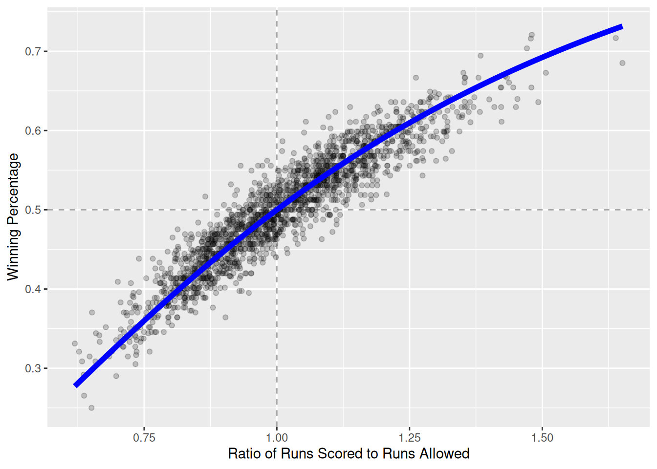
As noted in Section 4.2, one of the more enduring models in sabermetrics is Bill James’s formula for estimating a team’s expected winning percentage, given knowledge only of the team’s runs scored and runs allowed to date (recall that the team that scores the most runs wins a given game). This statistic is known—unfortunately—as Pythagorean Winning Percentage, even though it has nothing to do with Pythagoras. The formula is simple, but non-linear:
\[
\widehat{WPct} = \frac{RS^2}{RS^2 + RA^2} = \frac{1}{1 + (RA/RS)^2} \,,
\] where \(RS\) and \(RA\) are the number of runs the team has scored and allowed, respectively. If we define \(x = RS/RA\) to be the team’s run ratio, then this is a function of one variable having the form \(f(x) = \frac{1}{1 + (1/x)^2}\).
This model seems to fit quite well upon visual inspection—in Figure 7.1 we show the data since 1954, along with a line representing the model. Indeed, this model has also been successful in other sports, albeit with wholly different exponents.
exp_wpct <-function(x) { return(1/(1+ (1/x)^2))}TeamRuns <- Teams |>filter(yearID >=1954) |>rename(RS = R) |>mutate(WPct = W / (W + L), run_ratio = RS/RA) |>select(yearID, teamID, lgID, WPct, run_ratio)ggplot(data = TeamRuns, aes(x = run_ratio, y = WPct)) +geom_vline(xintercept =1, color ="darkgray", linetype =2) +geom_hline(yintercept =0.5, color ="darkgray", linetype =2) +geom_point(alpha =0.2) +stat_function(fun = exp_wpct, linewidth =2, color ="blue") +xlab("Ratio of Runs Scored to Runs Allowed") +ylab("Winning Percentage")
Figure 7.1: Fit for the Pythagorean Winning Percentage model for all teams since 1954.
However, the exponent of 2 was posited by James. One can imagine having the exponent become a parameter \(k\), and trying to find the optimal fit. Indeed, researchers have found that in baseball, the optimal value of \(k\) is not 2, but something closer to 1.85 (Wang 2006). It is easy enough for us to find the optimal value using the nls() function. We specify the formula of the nonlinear model, the data used to fit the model, and a starting value for the search.
Furthermore, researchers investigating this model have found that the optimal value of the exponent varies based on the era during which the model is fit. We can use the group_modify() function to do this for all decades in baseball history. First, we must write a short function (see Appendix C) that will return a data frame containing the optimal exponent, and for good measure, the number of observations during that decade.
fit_k <-function(x) { mod <-nls(formula = WPct ~1/(1+ (1/run_ratio)^k), data = x,start =list(k =2) )return(tibble(k =coef(mod), n =nrow(x)))}
Note that this function will return the optimal value of the exponent over any time period.
fit_k(TeamRuns)
# A tibble: 1 × 2
      k     n
  <dbl> <int>
1  1.83  1798
Finally, we compute the decade for each year using mutate(), define the group using group_by(), and apply fit_k() to those decades. The use of the ~ tells R to interpret the expression in parentheses as a formula, rather than the name of a function. The .x is a placeholder for the data frame for a particular decade.
Note the variation in the optimal value of \(k\). Even though the exponent is not the same in each decade, it varies within a fairly narrow range between 1.69 and 1.94.
7.5.2 Example: Annual leaders
As a second example, consider the problem of identifying the team in each season that led their league in home runs. We can easily write a function that will, for a specific year and league, return a data frame with one row that contains the team with the most home runs.
hr_leader <-function(x) {# x is a subset of Teams for a single year and league x |>select(teamID, HR) |>arrange(desc(HR)) |>head(1)}
Teams |>filter(yearID ==1961& lgID =="AL") |>hr_leader()
  teamID  HR
1    NYA 240
We can use group_modify() to quickly find all the teams that led their league in home runs. Here, we employ the .keep argument so that the grouping variables appear in the computation.
hr_leaders <- Teams |>group_by(yearID, lgID) |>group_modify(~hr_leader(.x), .keep =TRUE)tail(hr_leaders, 4)
# A tibble: 4 × 4
# Groups:   yearID, lgID [4]
  yearID lgID  teamID    HR
   <int> <fct> <fct>  <int>
1   2022 AL    NYA      254
2   2022 NL    ATL      243
3   2023 AL    MIN      233
4   2023 NL    ATL      307
In this manner, we can compute the average number of home runs hit in a season by the team that hit the most.
# A tibble: 2 × 2
  lgID  mean_hr
  <fct>   <dbl>
1 AL       176.
2 NL       163.
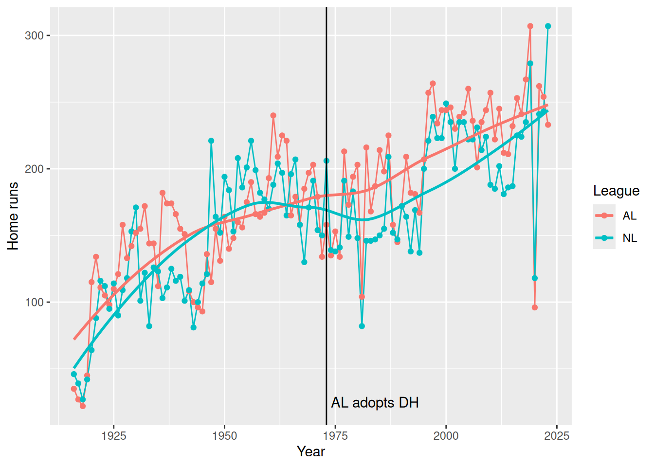
In Figure 7.2, we show how this number has changed over time. We note that while the top HR hitting teams were comparable across the two leagues until the mid-1970s, the AL teams have dominated since their league adopted the designated hitter rule in 1973.
hr_leaders |>filter(yearID >=1916) |>ggplot(aes(x = yearID, y = HR, color = lgID)) +geom_line() +geom_point() +geom_smooth(se =FALSE) +geom_vline(xintercept =1973) +annotate("text", x =1974, y =25, label ="AL adopts DH", hjust ="left" ) +labs(x ="Year", y ="Home runs", color ="League")
Figure 7.2: Number of home runs hit by the team with the most home runs, 1916–2019. Note how the AL has consistently bested the NL since the introduction of the designated hitter (DH) in 1973.
7.6 Simulation
In the previous section, we learned how to repeat operations while iterating over the elements of a vector. It can also be useful to simply repeat an operation many times and collect the results. Obviously, if the result of the operation is deterministic (i.e., you get the same answer every time) then this is pointless. On the other hand, if this operation involves randomness, then you won’t get the same answer every time, and understanding the distribution of values that your random operation produces can be useful. We will flesh out these ideas further in Chapter 13.
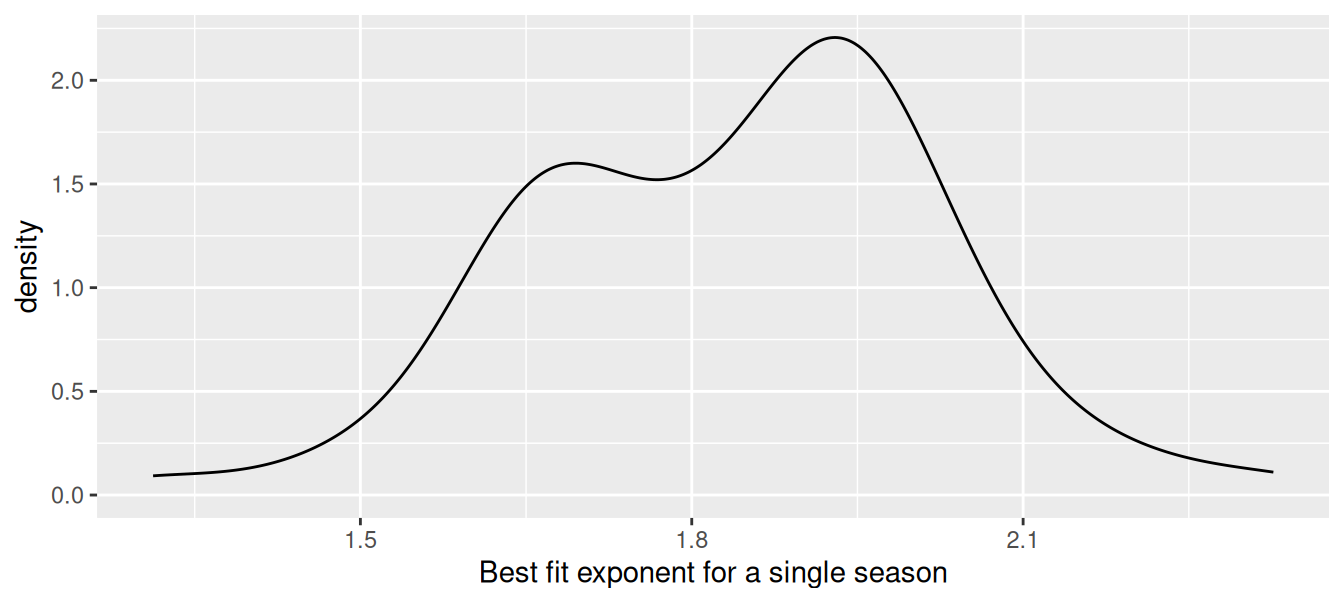
For example, in our investigation into the expected winning percentage in baseball (Section 7.5.1), we determined that the optimal exponent fit to the 66 seasons worth of data from 1954 to 2019 was 1.84. However, we also found that if we fit this same model separately for each decade, that optimal exponent varies from 1.69 to 1.94. This gives us a rough sense of the variability in this exponent—we observed values between 1.6 and 2, which may give some insights as to plausible values for the exponent.
Nevertheless, our choice to stratify by decade was somewhat arbitrary. A more natural question might be: What is the distribution of optimal exponents fit to a single-season’s worth of data? How confident should we be in that estimate of 1.84?
We can use group_modify() and the function we wrote previously to compute the 66 actual values. The resulting distribution is summarized in Figure 7.3.
── Variable type: numeric ──────────────────────────────────────────────────────
  var  n na mean    sd   p0  p25  p50  p75 p100
1 k   70  0 1.84 0.184 1.31 1.69 1.87 1.96 2.33
ggplot(data = k_actual, aes(x = k)) +geom_density() +xlab("Best fit exponent for a single season")
Figure 7.3: Distribution of best-fitting exponent across single seasons from 1954–2019.
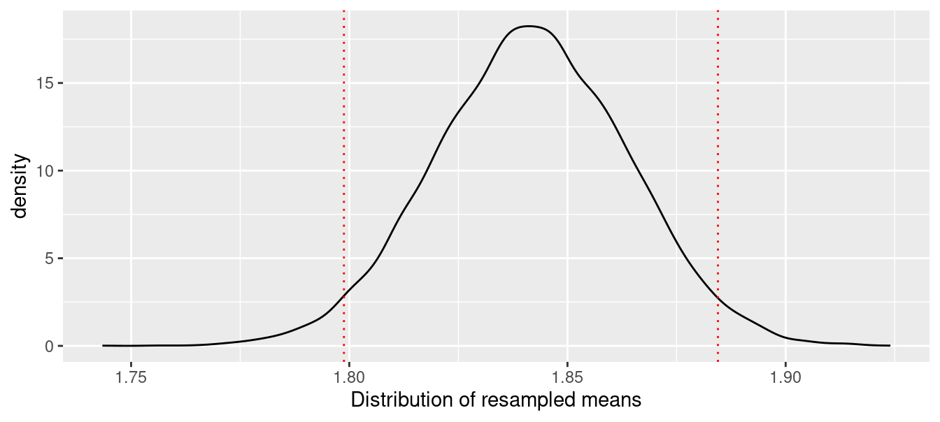
Since we only have 70 samples, we might obtain a better understanding of the sampling distribution of the mean \(k\) by resampling—sampling with replacement—from these 70 values. (This is a statistical technique known as the bootstrap, which we describe further in Chapter 9.) A simple way to do this is by mapping a sampling expression over an index of values. That is, we define n to be the number of iterations we want to perform, write an expression to compute the mean of a single resample, and then use map_dbl() to perform the iterations.
After repeating the resampling 10,000 times, we found that 95% of the resampled exponents were between 1.7975544 and 1.882597, with our original estimate of 1.84 lying somewhere near the center of that distribution. This distribution, along the boundaries of the middle 95%, is depicted in Figure 7.4.
ggplot(data =enframe(bstrap, value ="k"), aes(x = k)) +geom_density() +xlab("Distribution of resampled means") +geom_vline(data =enframe(civals), aes(xintercept = value), color ="red", linetype =3 )
Figure 7.4: Bootstrap distribution of mean optimal Pythagorean exponent.
7.7 Extended example: Factors associated with BMI
Body Mass Index (BMI) is a common measure of a person’s size, expressed as a ratio of their body’s mass to the square of their height. What factors are associated with high BMI?
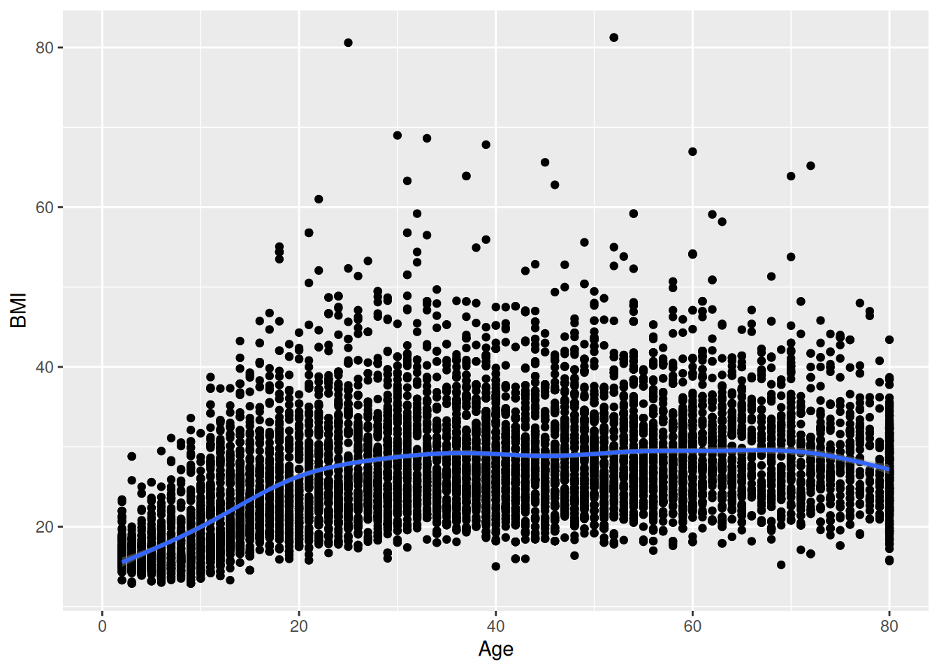
An exhaustive approach to understanding the relationship between BMI and some of the other variables is complicated by the fact that there are 75 potential explanatory varibles for any model for BMI. In Chapter 11, we develop several modeling techniques that might be useful for this purpose, but here, we focus on examining the bivariate relationships between BMI and the other explanatory variables. For example, we might start by simply producing a bivariate scatterplot between BMI and age, and adding a local regression line to show the general trend. Figure 7.5 shows the result.
ggplot(NHANES, aes(x = Age, y = BMI)) +geom_point() +geom_smooth()
Figure 7.5: Relationship between body mass index (BMI) and age among participants in the NHANES data.
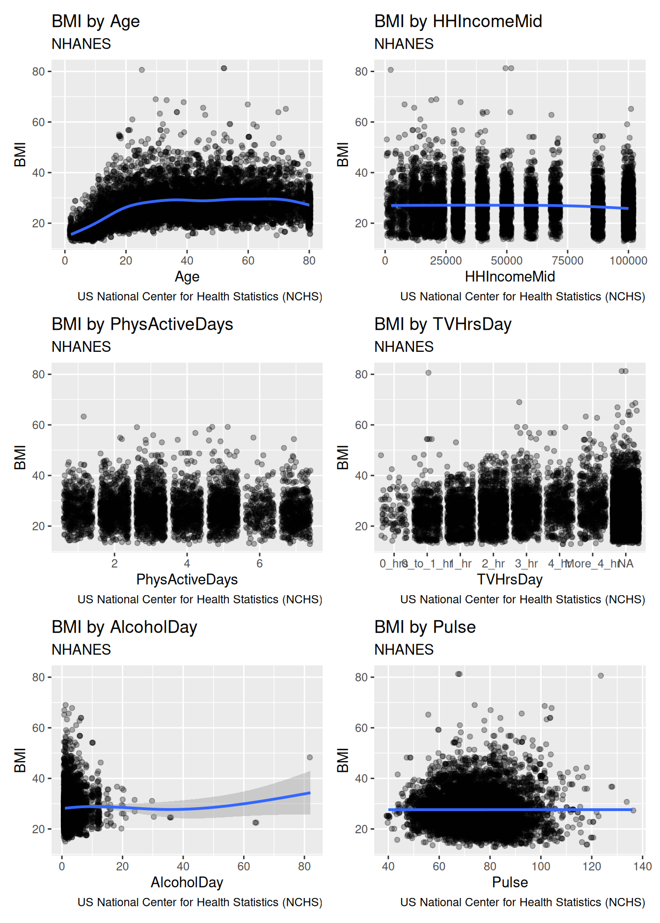
How can we programmatically produce an analogous image for all of the variables in NHANES? First, we’ll write a function that takes the name of a variable as an input, and returns the plot. Second, we’ll define a set of variables, and use map() to iterate our function over that list.
The following function will take a data set, and an argument called x_var that will be the name of a variable. It produces a slightly jazzed-up version of Figure 7.5 that contains variable-specific titles, as well as information about the source.
bmi_plot <-function(.data, x_var) {ggplot(.data, aes(y = BMI)) +aes_string(x = x_var) +geom_jitter(alpha =0.3) +geom_smooth() +labs(title =paste("BMI by", x_var),subtitle ="NHANES",caption ="US National Center for Health Statistics (NCHS)" )}
The use of the aes_string() function is necessary for ggplot2 to understand that we want to bind the x aesthetic to the variable whose name is stored in the x_var object, and not a variable that is named x_var!3
We can then call our function on a specific variable.
bmi_plot(NHANES, "Age")
Or, we can specify a set of variables and then map() over that set. Since map() always returns a list, and a list of plots is not that useful, we use the wrap_plots() function from the patchwork package to combine the resulting list of plots into one image.
Figure 7.6: Relationship between body mass index (BMI) and a series of other variables, for participants in the NHANES study.
Figure 7.6 displays the results for six variables. We won’t show the results of our ultimate goal to produce all 75 plots here, but you can try it for yourself by using the names() function to retrieve the full list of variable names. Or, you could use across() to retrieve only those variables that meet a certain condition.
7.8 Further resources
The chapter on functionals in Wickham (2019) is the definitive source for understanding purrr. The name “functionals” reflects the use of a programming paradigm called functional programming.
For those who are already familiar with the *apply() family of functions popular in base R, Jenny Bryan wrote a helpful tutorial that maps these functions to their purrr equivalents.
The rlang package lays the groundwork for tidy evaluation, which allows you to work programmatically with unquoted variable names. The programming with dplyr vignette is the best place to start learning about tidy evaluation. Section C.4 provides a brief introduction to the principles.
7.9 Exercises
Problem 1 (Easy): Use the HELPrct data from the mosaicData to calculate the mean of all numeric variables (be sure to exclude missing values).
Problem 2 (Easy): Suppose you want to visit airports in Boston (BOS), New York (JFK, LGA), San Francisco (SFO), Chicago (ORD, MDW), and Los Angeles (LAX). You have data about flight delays in a tibble called flights. You have written a pipeline that, for any given airport code (e.g., LGA), will return a tibble with two columns, the airport code, and the average arrival delay time.
Suggest a workflow that would be most efficient for computing the average arrival delay time for all seven airports.
Problem 3 (Medium): Use routines from the purrr package and the HELPrct data frame from the mosaicData package to fit a regression model predicting cesd as a function of age separately for each of the levels of the substance variable. Generate a formatted table (with suitable caption) of results (estimates and confidence intervals) for the slope parameter for each level of the grouping variable.
(Hint: Use group_by() and group_modify() to fit the regression model on each part. Note that broom::tidy() is useful in having the output of the model be a data frame.)
Problem 4 (Medium): The team IDs corresponding to Brooklyn baseball teams from the Teams data frame from the Lahman package are listed below. Use map_int() to find the number of seasons in which each of those teams played by calling a function called count_seasons.
Problem 5 (Medium): Use data from the NHANES package to create a set of scatterplots of Pulse as a function of Age, BMI, TVHrsDay, and BPSysAve to create a figure like the last one in the chapter. Be sure to create appropriate annotations (source, survey name, variables being displayed). What do you conclude?
Problem 6 (Hard): Use the group_modify() function and the Lahman data to replicate one of the baseball records plots (http://tinyurl.com/nytimes-records) from the The New York Times.
Wang, Victor. 2006. “The OBP/SLG Ratio: What Does History Say?”By the Numbers 16 (3): 3.
Wickham, H. 2019. Advanced r (Second Edition). CRC Press: Boca Raton, FL.
This works because a data frame is stored as a list of vectors of the same length. When you supply a data frame as the first argument to map(), you are giving map() a list of vectors, and it iterates a function over that list.↩︎
The plain function map() will always return a list.↩︎
Note that we use the quoted variable names here. To get this to work with unquoted variable names, see the Programming with dplyr vignette.↩︎